


The author, Meghan Cain, is a senior statistician, StataCorp.
Despite its explosive popularity in most fields over the last 20 years, machine learning remains underutilized in psychology. Although machine learning is often overlooked because psychologists are more interested in explaining behavior rather than predicting it, there are many outcomes in our field that it would be incredibly useful to predict, including suicide, Alzheimer’s or other degenerative diseases, dropping out of high school, divorce, or drug relapse. For example, you may collect data from patients before they leave a drug rehab program. Later, you may collect information on which patients relapsed. You could train a machine learning model on this dataset and use it to predict which patients are most at risk for relapse in the future.
Tree-based classifiers are among the most popular machine learning tools available for these type of classification problems. The simplest example of a tree-based classifier is a single decision tree, the goal of which is to split the sample into homogenous groups of the outcome variable based on a series of comparisons (see the decision tree in Figure 1). This is an oversimplified decision tree a banker might use to predict whether a potential client will repay their loan: “Yes” they will repay it or “No” they won’t. The first node, represented by a circle, compares clients’ credit scores to 600. Clients with a lower score are directed to a terminal node with prediction “No.” Clients with a higher score arrive at the next node, where they are split into two groups depending on their income. Clients with low income are directed to a terminal node with prediction “No,” and clients with high incomes are directed to a terminal node with prediction “Yes.”
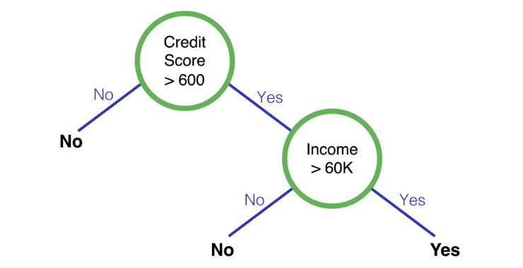
Figure 1: An example of a decision tree.
Decision trees are quick to estimate, easy to understand, and accurate within the dataset they are fit to, but their results don’t often generalize to new datasets. This is a problem called overfitting. Overfitting occurs when an overly complex model is fit too closely to a particular dataset, explaining that dataset’s idiosyncrasies instead of describing trends that are likely to occur across datasets.
To overcome the problem of overfitting, an ensemble of many decision trees can be grown, and their results can be aggregated together to form one final prediction. This is the idea behind random forest (Breiman, 2001), an ensemble learning method. In a random forest of decision trees, each tree is independently built using a random bootstrap sample drawn with replacement from the original dataset of the same sample size. Within each tree, a random subset of predictors is considered to determine the best split at each node. Performance increases as more trees are added, to a limit. Final predictions are made either by voting or averaging predictions across all trees. A ranking of the most important predictors used across trees can also be obtained.
Random forests require tuning of several parameters, including the number of predictors considered to create each split, the maximum number of nodes (interaction depth), and the minimum terminal node sample size. Tuning is always the most time-consuming part of machine learning. It’s generally a good idea to start with the default values in the software package you’re using, adding a smaller and larger value to test for each parameter. The entire set of parameters is evaluated according to some criterion, such as accuracy, AUC (WHAT ACRONYM IS THIS?), or mean square error, then the range of parameter values is repeatedly adjusted until a combination of values for all parameters is found that maximizes the criterion. The number of trees can be increased until the criterion is no longer appreciably improved.
In random forest, tuning is usually evaluated through out-of-bag error (OOB). Because each tree is built using a bootstrap sample with replacement, only about two-thirds of observations from the original dataset are used to create each tree. The accuracy of classifying each observation can be tested based on the trees that were created without that observation. This way, you don’t need to split your data into a training and testing set. The bootstrap procedure innately does that for you.
The predictive performance of random forest is very good, but the performance of a method called gradient boosting machines (GBM; Friedman, 2001) is often even better. The GBM algorithm minimizes a loss function using an ensemble of trees in a procedure similar to random forest. Trees are built sequentially to predict the remaining R-squared or pseudo R-squared of the specified loss function. The loss function could be binomial for binary data or mean square error for continuous data, or any other of a wide range of loss functions. Customized loss functions can also be used.
In addition to tuning the maximum depth and the minimum node size, GBM additionally requires tuning of the bag fraction and the shrinkage rate. In GBM, bootstrap samples are drawn at a sample size that is the specified bag fraction as large as the original sample without replacement size. Bag fraction is usually set to 50% but can be adjusted. The shrinkage rate is the rate at which the loss function is updated. Decreasing the shrinkage rate adds considerable computation time, but improves the predictive accuracy of the model to a point. A shrinkage rate that’s too low can overfit the data if too many trees are grown. To overcome the possibility of overfitting the data, early stopping procedures utilizing OOB can be used to stop the algorithm at a lower number of trees than specified.
When properly used, GBM is the most powerful predictive model for classification problems, as evidenced by its number of Kaggle competition wins (Harasymiv, 2015). The performance of random forest is only shortly behind and is much easier to tune and understand. Both are powerfully predictive tools with a wide range of possible applications in psychology research and practice, such as identifying potential patients or clients who are most in need of an intervention, predicting personality or other characteristics based on writing samples, helping us understand how humans make decisions, and many more.
References
Breiman, L. (2001). Random forests. Machine learning, 45(1), 5-32
Friedman, J. H. (2001). Greedy function approximation: a gradient boosting machine. Annals of statistics, 1189-1232
Harasymiv, V. (2015, November 3). Lessons from 2MM machine learning models on Kaggle.com—Data Science Meetup—Nov 2nd, 2015. LinkedIn. https://www.linkedin.com/pulse/lessons-from-2mm-machine-learning-models-kagglecom-data-harasymiv/opens in new window
Disclaimer: The views and opinions expressed in this article are those of the author. They are not endorsed by and do not necessarily reflect the position of StataCorp LLC.